Fraud Detection ( Model Building with AI)

By this Blog one can easily build Fraud Detection Model using Different Algorithms

# Import all Necessary libraries and files from libraries

# We have used here Pandas,Numpy,scipy,seaborn,tensorflow,keras,sklears all labraries we are utilising for Model Building

# Pandas for Dataframe

# Numpy for numerical operation, Scipy for generation of Statistical data

# Tensorflow is used for Neural Network Model Building

# Keras Library used for Autoencoder and building Model on several Iterations.

# Also used Regularazation,PCA method.

import os

import pandas as pd

import numpy as np

import pickle

import matplotlib.pyplot as plt

from scipy import stats

import tensorflow as tf

import seaborn as sns

from pylab import rcParams

from sklearn.model_selection import train_test_split

from keras.models import Model, load_model

from keras.layers import Input, Dense

from keras.callbacks import ModelCheckpoint, TensorBoard

from keras import regularizers

# Load the Working Directory, where my Data file has stored.

os.chdir("D:\My ML Simulations\Linear Regression")

# Load the data set, It is availabel on Kaggle for free.

carddata = pd.read_csv('creditcard.csv')

# See the data set with Limit on only first 9 Rows.

carddata.head(n=9)

carddata.shape

# Is Null Method is used to find out any Null values in Data Set?

carddata.isnull().values.any()

# As we are building Model on Fraud Detection, Assign 1:Fraudulent Behavious and 0: Non(Normal Transaction)

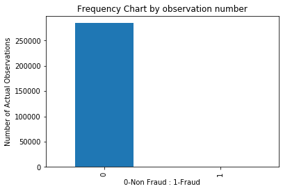
pd.value_counts(carddata['Class'], sort = True)

# Graphical Represantation of same data as Its easy way to understand.

count_classes = pd.value_counts(carddata['Class'], sort = True)

count_classes.plot(kind = 'bar', rot=90)

plt.xticks(range(2))

plt.title("Frequency Chart by observation number")

plt.xlabel("0-Non Fraud : 1-Fraud")

plt.ylabel("Number of Actual Observations");

normal_carddata = carddata[carddata.Class == 0]

Fraudulant_carddata = carddata[carddata.Class == 1]

# summary statistics differences between fraud and normal transactions.

# the mean is a little higher in the fraud transactions, it is certainly within a standard deviation and

# so is unlikely to be easy to discriminate in a highly precise manner between the classes with pure statistical methods.

normal_carddata.Amount.describe()

Fraudulant_carddata.Amount.describe()

bins = np.linspace(200, 2500, 100)

plt.hist(normal_carddata.Amount, bins, alpha=1, density=True, label='Normal Tx')

plt.hist(Fraudulant_carddata.Amount, bins, alpha=0.6, density=True, label='Fraud Tx')

plt.legend(loc='upper right')

plt.title("Amount by percentage of transactions (transactions \$200+)")

plt.xlabel("Transaction Amount in $ ")

plt.ylabel("Percentage of Transactions (%)");

plt.show()

# the fraud cases are relatively few in number compared to bin size,

# It would be hard to differentiate fraud from normal transactions by transaction amount alone.

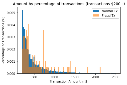
# The transaction amount does not look very informative. Let's look at the time of day:

bins = np.linspace(0, 48, 48) #48 hours

plt.hist((normal_carddata.Time/(60*60)), bins, alpha=1, density=True, label='Normal')

plt.hist((Fraudulant_carddata.Time/(60*60)), bins, alpha=0.6,density=True, label='Fraud')

plt.legend(loc='upper right')

plt.title("Percentage of transactions by hour")

plt.xlabel("Transaction time as measured from first transaction in the dataset (hours)")

plt.ylabel("Percentage of transactions (%)");

plt.hist((df.Time/(60*60)),bins)

plt.show()

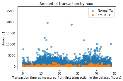
# Fraud tends to occur at higher rates during the night. Statistical tests could be used to give evidence for this fact.

plt.scatter((normal_carddata.Time/(60*60)), normal_carddata.Amount, alpha=0.6, label='Normal Tx')

plt.scatter((Fraudulant_carddata.Time/(60*60)), Fraudulant_carddata.Amount, alpha=0.9, label='Fraud Tx')

plt.title("Amount of transaction by hour")

plt.xlabel("Transaction time as measured from first transaction in the dataset (hours)")

plt.ylabel('Amount $')

plt.legend(loc='upper right')

plt.show()

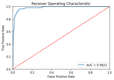
fpr, tpr, thresholds = roc_curve(error_carddata.true_class, error_carddata.reconstruction_error)

roc_auc = auc(fpr, tpr)

plt.title('Receiver Operating Characteristic')

plt.plot(fpr, tpr, label='AUC = %0.4f'% roc_auc)

plt.legend(loc='lower right')

plt.plot([0,1],[0,1],'r--')

plt.xlim([-0.001, 1])

plt.ylim([0, 1.001])

plt.ylabel('True Positive Rate')

plt.xlabel('False Positive Rate')

plt.show();

# Receiver operating characteristic curves are an expected output of most binary classifiers.

# Since we have an imbalanced data set they are somewhat less useful.

# Basically, we want the blue line to be as close as possible to the upper left corner.

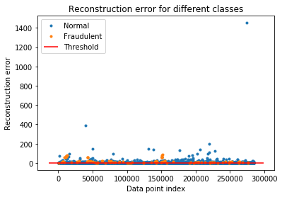
groups = error_carddata.groupby('true_class')

fig, ax = plt.subplots()

for name, group in groups:

ax.plot(group.index, group.reconstruction_error, marker='o', ms=3, linestyle='',

label= "Fraudulent" if name == 1 else "Normal")

ax.hlines(threshold, ax.get_xlim()[0], ax.get_xlim()[1], colors="r", zorder=100, label='Threshold')

ax.legend()

plt.title("Reconstruction Error For Different Classes")

plt.ylabel("Reconstruction error")

plt.xlabel("Data point index")

plt.show();

plt.figure(figsize=(8, 8))

sns.heatmap(conf_matrix,xticklabels='auto', yticklabels='auto',robust=False, annot= True, fmt="d");

plt.title("Confusion matrix")

plt.ylabel('True class')

plt.xlabel('Predicted class')

plt.show()

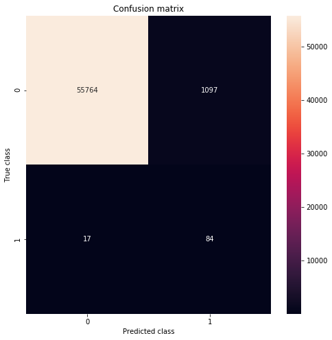
# Our model seems to catch a lot of the fraudulent cases. Of course, there is a catch.

# We might want to increase or decrease the value of the threshold, depending on the problem.

# I presented the business case for card payment fraud detection and provided a brief overview of the algorithms in use.